
I’ve been reading “The Book of Why” by Judea Pearl over the past few weeks, which has really helped formalize my intuition of causation. However, the book would be much better if Pearl left out any sentences written in the first-person as he has an annoying tendency to style himself as a messiah proclaiming the enlightened concepts of Causation to all the lowly statisticians still stuck on Correlation.
If we can look past his self-aggrandizing remarks, “The Book of Why” applies causal models to examples from the surgeon general’s committee on smoking in the 1960’s to the Monty Hall paradox. By reducing these multi-faceted problems down to a causal representation, we can finally put our finger on contributing factors or “causes” and control for them (if possible) to isolate the effect we are attempting to discover.
Perhaps the biggest takeaway for me from this book is the need to understand the data generation process when working with a dataset. This might sound like a no-brainer but too often, data scientists are so eager to jump in to the big shiny ball pit of a new dataset that they don’t stop to think about what this data actually represents.
Data scientists with a new dataset
By including the process by which the data was generated in these causal models, we can augment our own mental model and unlock the true relationships behind the variables of interest.
So what’s a DAG?
Directly acyclic graphs (DAG’s) are a visual representation of a causal model. Here’s a simple one:

You were late for work because you had to change your car’s tire because it was flat. Of course, we could add on much more than this (why was it flat?) but you get the idea.
Junction Types
Let’s explore what we can do with DAG’s through different junction types.
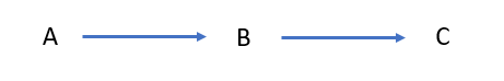
Chain
This is the simplest DAG and is represented in the example above. A generalized representation below shows that A is a cause of B, which is itself a cause of C.
Collider
Now we have two causes for C. Both A and B affect the outcome C.
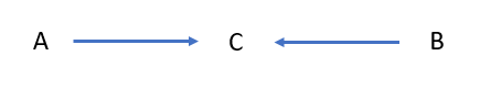
Conditioning on C will reveal a non-causal, negative correlation between A & B. This correlation is called collider bias.
We can understand this effect in crude mathematical terms. If A + B = C and we hold C constant, then we must increase A by the same amount we decrease B.
Additionally, this phenomenon is sometimes also called the “explain-away effect” because C “explains away” the correlation between A and B.
Note that the collider bias may be positive in cases when contributions from both A and B are necessary to affect C.
An example of a collider relationship would be the age-old nature vs. nurture question. Someone’s personality (C) is a product of both their upbringing (A) and the genes (B).
Fork
In the case of a fork, A affects both B and C.
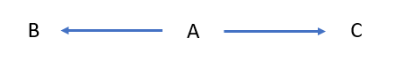
Without conditioning on A, there exists a spurious (non-causal) correlation between B & C. A classic example of a spurious correlation is the relationship between crime (B) and ice cream sales (C). When you plot these two values over time, they appear to increase and decrease together, suggesting some kind of causality. Does ice cream cause people to commit crime?
Of course, this relationship can be explained by adding in temperature (A). Warmer weather causes people to leave their homes more often, leading to more crime (B). People also crave ice cream cones (C) on hot days.
Node Types
Mediators
A mediator is the node that “mediates” or transmits a causal effect from one node to another.
Again using the example below, B mediates the causal effect of A onto C.
Confounders
Harking back to the crime-and-ice-cream example, temperature is the confounder node as it “confounds” the relationship between ice cream sales and crime.
If we control for the confounder (A), we can isolate the relationship between C and B, if one exists. This is a key concept for experimental design.
Correcting for Confounding
Let’s spend some more time on this subject. Pearl’s assertion is that if we control for all confounders, we should be able to isolate the relationship between the variables of interest and therefore prove causation, instead of mere correlation.
Pearl defines confounding more broadly as any relationship that leads to  , where the
  operator implies an action. In other words, if there is a difference between the probability of an outcome
  given
given  and the probability of given in a perfect world in which we were able to change and only , then confounding is afoot.
Four Rules of Information Flow
Pearl has 4 rules for controlling the flow of information through a DAG.
- In a chain (A → B → C), B carries information from A to C. Therefore, controlling for B prevents information about A from reaching C and vice versa.
- In a fork (A ← B → C), B is the only known common source of information between both A and C. Therefore, controlling for B prevents information about A from reaching C and vice versa.
- In a collider (A → B ← C), controlling for B “opens up” the pipe between A and C due to the explain-away effect.
- Controlling for descendants of a variable will partially control for the variable itself. Therefore, controlling the descendant of a mediator partially closes the pipe, and controlling for the descendant of a collider partially opens the pipe.
Back-door criterion
We can use these causal models as represented by DAG’s to determine how exactly we should remove this confounding from our study.
If we are interested in understanding the relationship between only X and Y, we must identify and dispatch any confounding back-door paths, where a back-door path is any path from X to Y that starts with an arrow into X.
Pearl’s Games
Pearl devises a series of games that involve increasingly complicated DAG’s where the objective is to “deconfound” the path from X to Y. This is achieved by blocking every non-causal path while leaving all causal paths intact.
In other words, we need to identify and block all back-door paths while ensuring that any variable Z on a back-door path is not a descendant of X via a causal path to Y.
Let’s go through some examples, using the numbered games from the book.
Game 2
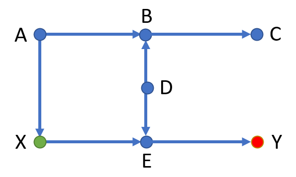
We need to determine which variables (if any) of A, B, C, D, or E need to be controlled in order to deconfound the path from X to Y.
There is one back-door path: X ← A → B ← D → E → Y. This path is blocked by the collider at B from the third rule of information flow.
Therefore, there is no need to control any of these variables!
Game 5
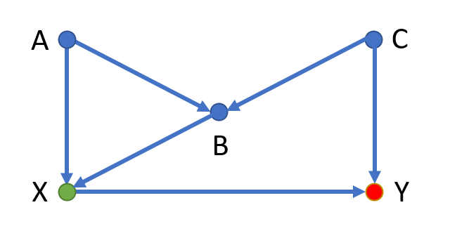
This one’s a bit more interesting. We have two back-door paths:
- X ← A → B ← C → Y
- X ← B ← C → Y
The first back-door path is blocked by a collider at B so there is no need to control any variables due to this relationship.
The second path, however, represents a non-causal path between X and Y. We need to control for either B or C.
But watch out! If we control for B, we fall into the condition outlined by Pearl’s third rule above, where we’ve controlled for a collider and thus opened up the first back-door path in this diagram.
Therefore, if we control for B, we will then have to control for A or C as well. However, we can also control for only C initially and avoid the collider bias altogether.
Conclusion
DAG’s can be an informative way to organize our mental models around causal relationships. Keeping in mind Pearl’s Four Rules of Information Flow, we can identify confounding variables that cloud the true relationship between the variables under study.
Bringing this home for data scientists, when we include the data generation process as a variable in a DAG, we remove much of the mystery surrounding such pitfalls as Simpson’s Paradox. We’re able to think more like informed humans and less like data-crunching machines—an ability we should all be striving for in our increasingly AI-driven world.