Mel Hanna

Precision and recall aren’t the only ways to quantify our performance when developing a classifier.

Plotting a Receiver Operating Characteristic (ROC) curve is another useful tool to help us quickly determine how well the classifier performs and visualize any trade-offs we might be making as we attempt to balance Type I and Type II error rates.

The basics

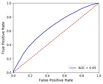
Let’s jump right in. Here’s an ROC curve for a model that predicts credit card default (where a positive is considered to be a default).

Axes

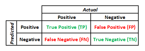
The x-axis represents the False Positive Rate (FPR) or the probability of a false alarm. This can be calculated through:

Put another way, FPR represents the fraction of incorrectly classified negatives (in this case, accounts that did not default but for which our model predicted would default) within the total population of negatives (all accounts that did not default).

The y-axis shows the True Positive Rate (TPR), which is equivalent to the recall.

Recall is just class-specific accuracy or:

Again, in the context of our example, this is the fraction of accounts that did default and for which our model predicted they would within the total population of accounts that did default.

The diagonal

The red dashed line dividing the plot represents random performance. When the FPR matches the TPR, we might as well be guessing–you’re right as often as you’re wrong.

If your curve falls to the left of the diagonal, the model is performing better than random because your true positive rate exceeds your false positive rate. Likewise, a curve to the right of the diagonal indicates some systemic error in your model, causing it to perform worse than random.

The curve

Now that we’ve established the space in which we’re working, we can best understand how to determine the ROC curve above.

The ROC visualizes the trade-offs between the FPR and the TPR when we adjust the threshold by which the classifier makes its determination.

For example, our model could determine a credit default using a probability threshold of 0.25. If the model’s probability of default is 0.32, we would return “default”. If the probability is 0.19, we could return “no default”.

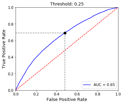
This is illustrated in the ROC plot above. The FPR and TPR for a threshold of 0.25 is represented by the black dot on the ROC curve. Our TPR is roughly 0.7 and our FPR is around 0.45.

Now, let’s lower the threshold to 0.15.

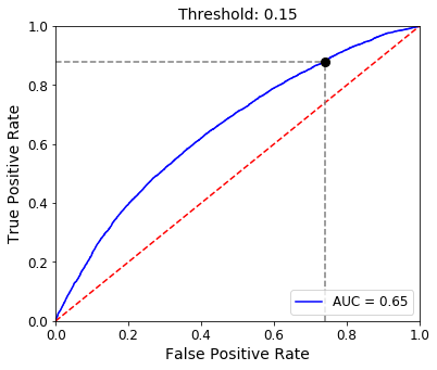
We move further up the curve, increasing our TPR to nearly 0.9 but also increasing our FPR to about 0.75.

This illustrates the principle that as we decrease our decision threshold, we move to the right and upwards along the curve because we are simply classifying more observations overall as positives. Therefore, TPR increases as we capture more of those true positives but at the same time, our probability of false alarm also goes up as we become less strict with our requirement to classify a positive.

Choosing a threshold

This observation begs the question–what would be the optimal threshold to choose?

Of course, this will likely depend on model-specific considerations. For example, what is the cost of a false positive? If it’s relatively low, we might as well increase our TPR at the expense of an increased FPR as well.

However, if we’d like to try and balance these two competing metrics, we can choose the point along the curve that is closest to the top-left corner of the plot. This could be considered the apex of the curve, as shown below.

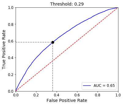
The apex can be found by determining where on the curve we find a maximum difference between TPR and FPR. In our case, this occurs at a threshold of 0.29 to return a TPR of nearly 0.6 and a FPR of about 0.36.

AUC

Perhaps the most widely used application of an ROC curve is to calculate the area underneath it. This is called AUC or “Area Under Curve”.

The area in gray below represents the AUC.

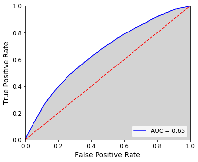
Our AUC for this model is 0.65. A random model would produce an AUC of 0.5 so we are doing better than guessing!

An ideal model would have an ROC curve that hugs the axes with an apex close to the upper-left corner, resulting in an AUC of nearly 1.0. Therefore, AUC is a way to quantify the ability of the model to maximize TPR while minimizing FPR, no matter the threshold chosen.

Congrats! You’ve built a binary classifier that you’re convinced is totally awesome.

But how do you quantify just how awesome this model is? And more specifically, how do you communicate this model’s level of awesomeness to your manager/product owner/stakeholder/random-person-on-the-street?

This is where performance metrics such as precision and recall come into play, and we’ll attempt to explain the intuition around these in addition to their definitions.

What is the positive class?

If you’ve built a binary classifier, perhaps the first step in determining your performance metric is to select a “positive” class. This is easy in some instances (ex. coronavirus test result) and less so in others (ex. determining if your pet is either a cat or a chinchilla). But establishing these definitions early (and stating them explicitly) will save a lot of confusion down the road.

False negatives vs. true positives

Something I struggled with initially was what exactly did we mean by a “false negative”? Was it a true negative that we classified incorrectly? Or did the model return an incorrect (and therefore false) prediction of negative? In other words, from whose perspective do we consider this classification false?

The answer is the latter definition above. The table below sums this up.

Confusion matrix

Once you’ve established your false positives and false negatives, you can display them in a confusion matrix that looks very similar to the table above.

Here is an example for a classifier that attempts to determine if shoplifting is taking place (where we define a shoplifting incident as a positive). Let’s say for example, this model takes video footage from a store surveillance system and looks for certain features (ex. a customer picking up an item and hiding it under his/her shirt) that would indicate shoplifting.

The confusion matrix shows the number of observations for each class and the corresponding predictions from the model.

From the matrix above, we can see that our classifier is rather paranoid and often mistakes normal behavior for shoplifting.

Accuracy

Now we can start to sum up the classifier’s performance using a single value, such as the accuracy, which represents the fraction of correct predictions out of the total. In the shoplifting example, the accuracy is shown by the following:

Wowza, this is a terrible model.

WARNING: Note that accuracy is a misleading metric in this case due to unbalanced class sizes.

In other words, because we have so few true shoplifting incidences compared to cases of normal behavior, we can easily achieve an accuracy of 0.904 by returning a prediction of “normal” every time. But no one would consider such a classifier to be truly “accurate”.

Precision and Recall

I mentioned earlier that our classifier tends to overpredict shoplifting–how can we incorporate this tendency into a performance metric?

This is where precision and recall come into play. These metrics are class-specific, which means that we must specify a value for both precision and recall for each class returned by the model.

Precision

Precision is the answer to the question: out of the total predictions for a certain class returned by the model, how many were actually correct? For example, the precision for the shoplifting class is:

Similarly, for the normal behavior:

In other words, the model’s predictions for normal behavior were correct 93% of the time, while its predictions for shoplifting were correct only 10% of the time. Yikes.

Recall

I like to think of recall as a class-specific accuracy. How many of the model’s predictions for a certain class were actually correct?

The model correctly identified 83% of the actual shoplifting incidents.

And here we see the trade-off often inherent in precision and recall. The model correctly predicted a good majority (83%) of the actual shoplifting incidents, but at the expense of also erroneously predicting many truly normal behaviors as shoplifting too (nearly 90% of the predicted shoplifting incidents).

This ties into Type I and Type II errors, where a type I error is a false positive (normal behavior incorrectly classified as shoplifting) and a type II error is a false negative (shoplifting incorrectly classified as normal behavior).

For our situation, this boils down to asking if you would rather have the police called on an innocent customer (type I) or lose merchandise to unchecked shoplifters (type II)?

Understanding the costs of type I and type II errors helps to weigh whether you’d like to improve either recall or precision. Often, it’s difficult to do both simultaneously.

F1-Score

However, if you’d like to tie up both precision and recall into one single metric to hand over to your manager/product owner/stakeholder, then the F1-score (sometimes called F-measure) is for you!

This is simply the harmonic mean of the precision and recall for a given class, shown below.

An F1-score of 1 indicates perfect precision and recall.

If you’d like to place more importance on recall over precision, you can introduce a term (set to a value less than 1 to place more emphasis of precision instead of recall).