Classifying Labradors with fastai

Although I’ve been a practicing data scientist for more than three years, deep learning remained an enigma to me. I completed Andrew Ng’s deep learning specialization on Coursera last year but while I came away with a deeper understanding of the mathematical underpinnings of neural networks, I could not for the life of me build one myself.

Enter fastai. With a mission to “make neural nets uncool again”, fastai hands you all the tools to build a deep learning model today. I’ve been working my way through their MOOC, Practical Deep Learning for Coders, one week at a time and reading the corresponding chapters in the book.

I really appreciate how the authors jump right in and ask you to get your hands dirty by building a model using their highly abstracted library (also called fastai). An education in the technical sciences too often starts with the nitty gritty fundamentals and abstruse theories and then works its way up to real-life applications. By this time, of course, most of the students have thrown their hands up in despair and dropped out of the program. The way fastai approaches teaching deep learning is to empower its students right off the bat with the ability to create a working model and then to ask you to look under the hood to understand how it operates and how we might troubleshoot or fine-tune our performance.

A brief introduction to Labradors

To follow along with the course, I decided to create a labrador retriever classifier. I have an American lab named Sydney, and I thought the differences between English and American labs might pose a bit of a challenge to a convolutional neural net since the physical variation between the two types of dog can often be subtle.

Some history

At the beginning of the 20th century, all labs looked similar to American labs. They were working dogs and needed to be agile and athletic. Around the 1940’s, dog shows became popular, and breeders began selecting labrador retrievers based on appearance, eventually resulting in what we call the English lab. English labs in England are actually called “show” or “bench” labs, while American labs over the pond are referred to as working Labradors.

Nowadays, English labs are more commonly kept as pets while American labs are still popular with hunters and outdoorsmen.

Physical differences

English labs tend to be shorter in height and wider in girth. They have shorter snouts and thicker coats. American labs by contrast are taller and thinner with a longer snout.

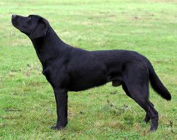
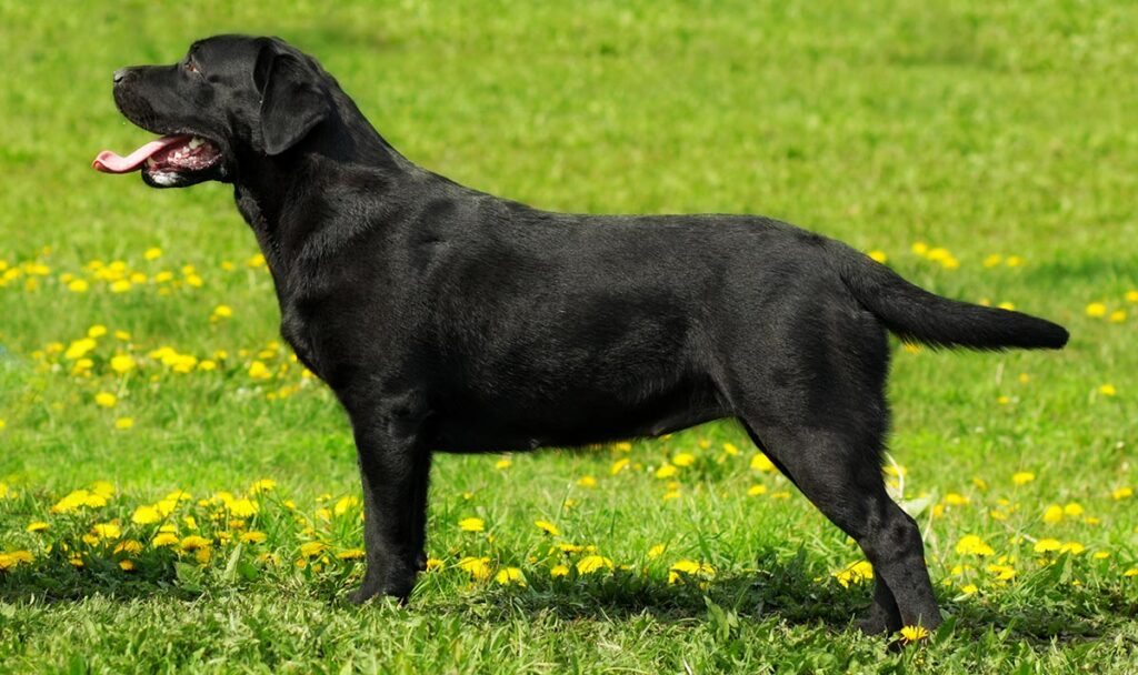
These differences may not be stark as both are still Labrador Retrievers and are not bred to a standard.

Gathering data

First we need images of both American and English labs on which to train our model. The fastai course leverages the Bing Image Search API through MS Azure. The code below shows how I downloaded 150 images each of English and American labrador retrievers and stored them in respective directories.

path = Path('/storage/dogs')

subscription_key = "" # key obtained through MS Azure
search_url = "https://api.bing.microsoft.com/v7.0/images/search"
headers = {"Ocp-Apim-Subscription-Key" : subscription_key}

names = ['english', 'american']

if not path.exists():
    path.mkdir()
for o in names:
    dest = (path/o)
    dest.mkdir(exist_ok=True)

    params  = {
        "q": '{} labrador retriever'.format(o),
        "license": "public",
        "imageType": "photo",
        "count":"150"
    }

    response = requests.get(search_url, headers=headers, params=params)
    response.raise_for_status()
    search_results = response.json()

    img_urls = [img['contentUrl'] for img in search_results["value"]]

    download_images(dest, urls=img_urls)

Let’s check if any of these files are corrupt.

fns_updated = get_image_files(path)
failed = verify_images(fns)
failed

(#1) [Path('/storage/dogs/english/00000133.svg')]

We’ll remove that corrupt file from our images.

failed.map(Path.unlink);

First model attempt

I create a function to process the data using a fastai class called DataBlock, which does the following:

• Defines the independent data as an ImageBlock and the dependent data as a CategoryBlock
  
  
• Retrieves the data using a fastai function get_image_files from a given path
  
  
• Splits the data randomly into a 20% validation set and 80% training set
  
  
• Attaches the directory name (“english”, “american”) as the image labels
  
  
• Crops the images to a uniform 224 pixels by randomly selecting certain 224 pixel areas of each image, ensuring a minimum of 50% of the image is included in the crop. This random cropping repeats for each epoch to capture different pieces of the image.

def process_dog_data(path):
    dogs = DataBlock(
        blocks=(ImageBlock, CategoryBlock), 
        get_items=get_image_files, 
        splitter=RandomSplitter(valid_pct=0.2, seed=44),
        get_y=parent_label,
        item_tfms=RandomResizedCrop(224, min_scale=0.5)
    )

    return dogs.dataloaders()

The item transformation (RandomResizedCrop) is an important design consideration. We want to use as much of the image as possible while ensuring a uniform size for processing. But in the process of naive cropping, we may be omitting pieces of the image that are important for classification (ex. the dog’s snout). Padding the image may help but wastes computation for the model and decreases resolution on the useful parts of the image.

Another approach of resizing the image (instead of cropping) results in distortions, which is especially problematic for our use case as the main differences between English and American labs is in their proportions. Therefore, we settle on the random cropping approach as a compromise. This strategy also acts as a data augmentation technique by providing different “views” of the same dog to the model.

Now we “fine-tune” ResNet-18, which replaces the last layer of the original ResNet-18 with a new random head and uses one epoch to fit this new model on our data. Then we fit this new model for the number of epochs requested (in our case, 4), updating the weights of the later layers faster than the earlier ones.

dls = process_dog_data(path)

learn = cnn_learner(dls, resnet18, metrics=error_rate)
learn.fine_tune(4)

epoch	train_loss	valid_loss	error_rate	time
0	1.392489	0.944025	0.389831	00:15

epoch	train_loss	valid_loss	error_rate	time
0	1.134894	0.818585	0.305085	00:15
1	1.009688	0.807327	0.322034	00:15
2	0.898921	0.833640	0.338983	00:15
3	0.781876	0.854603	0.372881	00:15

These numbers are not exactly ideal. While training and validation loss mainly decrease, our error rate is actually increasing.

interp = ClassificationInterpretation.from_learner(learn)
interp.plot_confusion_matrix(figsize=(5,5))

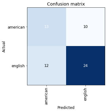
The confusion matrix shows poor performance, especially on American labs. We can take a closer look at our data using fastai’s ImageClassifierCleaner tool, which displays the images with the highest loss for both training and validation sets. We can then decide whether to delete these images or move them between classes.

cleaner = ImageClassifierCleaner(learn)
cleaner

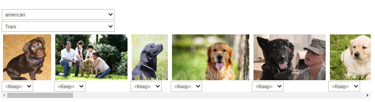
We definitely have a data quality problem here as we can see that the fifth photo from the left is a German shepherd and the fourth photo (and possibly the second) is a golden retriever.

We can tag these kinds of images for removal and retrain our model.

After data cleaning

Now I’ve gone through and removed 49 images from the original 300 that were not the correct classifications of American or English labs. Let’s see how this culling has affected performance.

dls = process_dog_data()

learn = cnn_learner(dls, resnet18, metrics=error_rate)
learn.fine_tune(4)

epoch	train_loss	valid_loss	error_rate	time
0	1.255060	0.726968	0.380000	00:14

epoch	train_loss	valid_loss	error_rate	time
0	0.826457	0.670593	0.380000	00:14
1	0.797378	0.744757	0.320000	00:15
2	0.723976	0.809631	0.260000	00:15
3	0.660038	0.849696	0.280000	00:13

Already we see improvement in that our error rate is finally decreasing for each epoch, although our validation loss increases.

interp = ClassificationInterpretation.from_learner(learn)
interp.plot_confusion_matrix(figsize=(5,5))

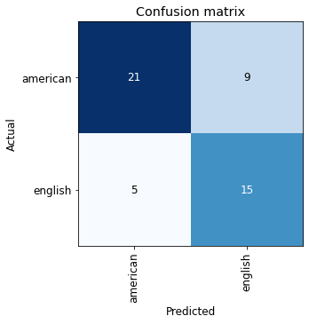
This confusion matrix shows much better classification for both American and English labs.

Now let’s see how this model performs on a photo of my own dog.

Using the Model for Inference

I’ll upload a photo of my dog Sydney.

btn_upload = widgets.FileUpload()
btn_upload

img = PILImage.create(btn_upload.data[-1])
out_pl = widgets.Output()
out_pl.clear_output()
with out_pl: display(img.rotate(270).to_thumb(128,128))
out_pl

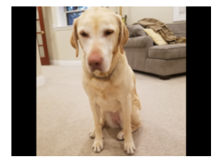
This picture shows her elongated snout and sleeker body, trademarks of an American lab.

pred,pred_idx,probs = learn.predict(img)
lbl_pred = widgets.Label()
lbl_pred.value = f'Prediction: {pred}; Probability: {probs[pred_idx]:.04f}'
lbl_pred

Label(value='Prediction: american; Probability: 0.9284')

The model got it right!

Take-aways

Data quality

If I were serious about improving this model, I’d manually look through all these images to confirm that they contain either English or American labs. Based on the images shown by the cleaner tool, the Bing Image Search API does not return many relevant results and needs to be supervised closely.

Data quantity

I was definitely surprised to achieve such decent performance on so few images. I had always been under the impression that neural networks required a lot of data to avoid overfitting. Granted, this may still be the case here based on the growing validation loss but I’m looking forward to learning more about this aspect later in the course.

fastai library

While I appreciate that the fastai library is easy-to-use and ideal for deep learning beginners, I found some of the functionality too abstracted at times and difficult to modify or troubleshoot. I suspect that subsequent chapters will help me become more familiar with the library and feel more comfortable making adjustments but for someone used to working more with the nuts and bolts within Python, this kind of development felt like a loss of control.

Model explainability

I’m extremely interested to understand how the model arrives at its classifications. Is the model picking up on the same attributes that humans use to classify these dogs (i.e. snouts, body shapes)? While I’m familiar with the SHAP library and its ability to highlight CNN feature importances within images, Chapter 18 of the book introduces “class activation maps” or CAM’s to accomplish the same goal. I’ll revisit this model once I’ve made further progress in the course to apply some of these explanability techniques to our Labrador classifier and understand what makes it tick.